
Plot gallery
Build retained multi-axis figures, render them through OA’s Vulkan compositor, and reproduce six checked presentation assets from matching C++ and Python programs.
TuPaired source6 outputsUi
Source
| Surface | Repository path | SHA-256 |
|---|---|---|
| C++ | sdk/cpp/tutorials/plot/tuPlotGallery.cpp | 0694b990fb1b8b76 |
| Python | sdk/py/tutorials/plot/tuPlotGallery.py | 8f3d7b1e1512e3e6 |
| Presentation | sdk/asset/docs/plot/*.png | Verified per image |
Example
A figure owns layout and axes state. Each axes records semantic artists; rendering lowers the retained figure through the shared compositor and returns an oa::Image. The language switch replaces the complete checked source fragment.
1oa::plot::Figure introFigure() {2 oa::plot::Figure figure({3 .title = "OA Plot intro",4 .rows = 1,5 .cols = 2,6 .width = 1280U,7 .height = 560U,8 .hSpacing = 36,9 .padding = 34,10 .theme = oa::plot::Theme::Dark,11 });12 figure.title("One retained figure - C++ and Python parity");1314 constexpr oa::Array<oa::F32, 8> steps{15 0.0F, 1.0F, 2.0F, 3.0F, 4.0F, 5.0F, 6.0F, 7.0F};16 constexpr oa::Array<oa::F32, 8> train{17 1.00F, 0.78F, 0.61F, 0.48F, 0.37F, 0.29F, 0.23F, 0.19F};18 constexpr oa::Array<oa::F32, 8> validation{19 1.04F, 0.83F, 0.66F, 0.53F, 0.43F, 0.35F, 0.30F, 0.27F};20 constexpr oa::Array<oa::F32, 5> ideal{21 0.0F, 0.25F, 0.50F, 0.75F, 1.0F};22 constexpr oa::Array<oa::F32, 5> confidence{23 0.10F, 0.30F, 0.50F, 0.70F, 0.90F};24 constexpr oa::Array<oa::F32, 5> accuracy{25 0.08F, 0.34F, 0.47F, 0.74F, 0.88F};2627 auto& curves = figure.ax(0, 0);28 curves.title("training curves");29 curves.xLabel("optimizer step");30 curves.yLabel("cross entropy");31 curves.limits(0.0F, 7.0F, 0.0F, 1.1F);32 curves.plot(steps, train,33 {.color = oa::Color::accent(), .label = "train", .width = 1.6F});34 curves.plot(steps, validation,35 {.color = oa::Color::success(), .label = "validation", .width = 1.6F});3637 auto& quality = figure.ax(0, 1);38 quality.title("Calibration");39 quality.xLabel("confidence");40 quality.yLabel("observed accuracy");41 quality.limits(0.0F, 1.0F, 0.0F, 1.0F);42 quality.plot(ideal, ideal,43 {.color = oa::Color{0.565F, 0.565F, 0.565F, 1.0F},44 .label = "ideal"});45 quality.scatter(confidence, accuracy,46 {.color = oa::Color::cyan(), .label = "model", .radius = 3.5F});47 return figure;48}49
Present
Six checked renders cover dark and light diagnostics, evaluation curves, dense training layouts, and projected scalar-field landscapes.
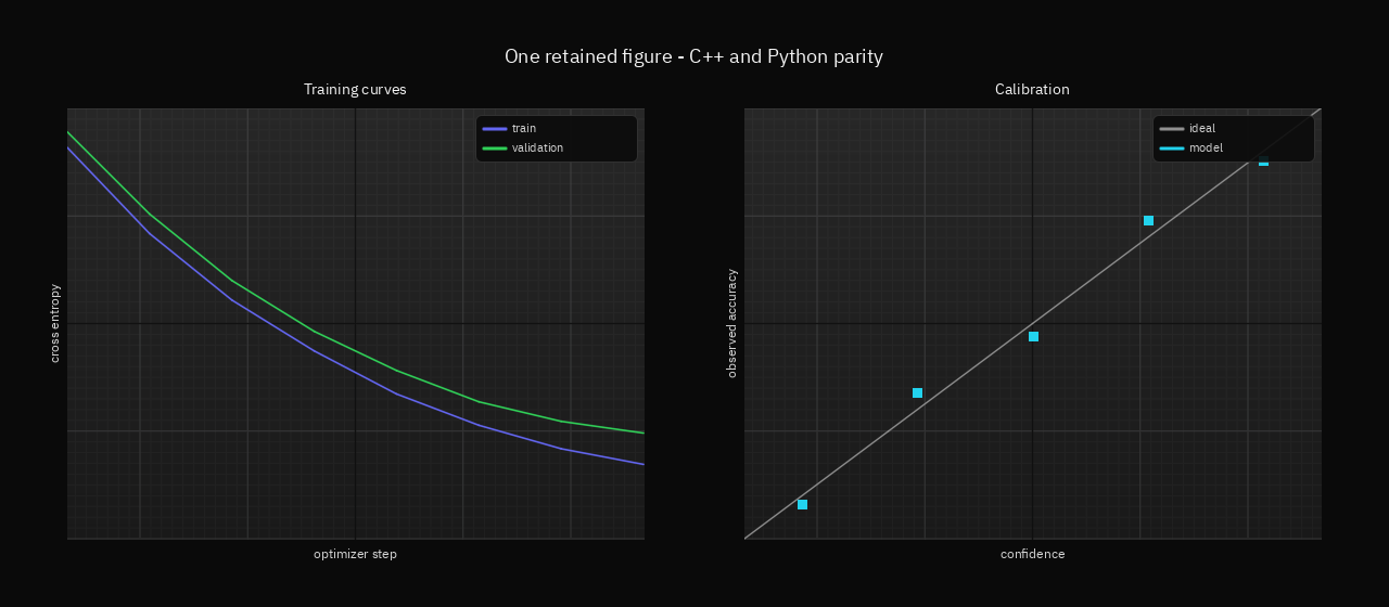
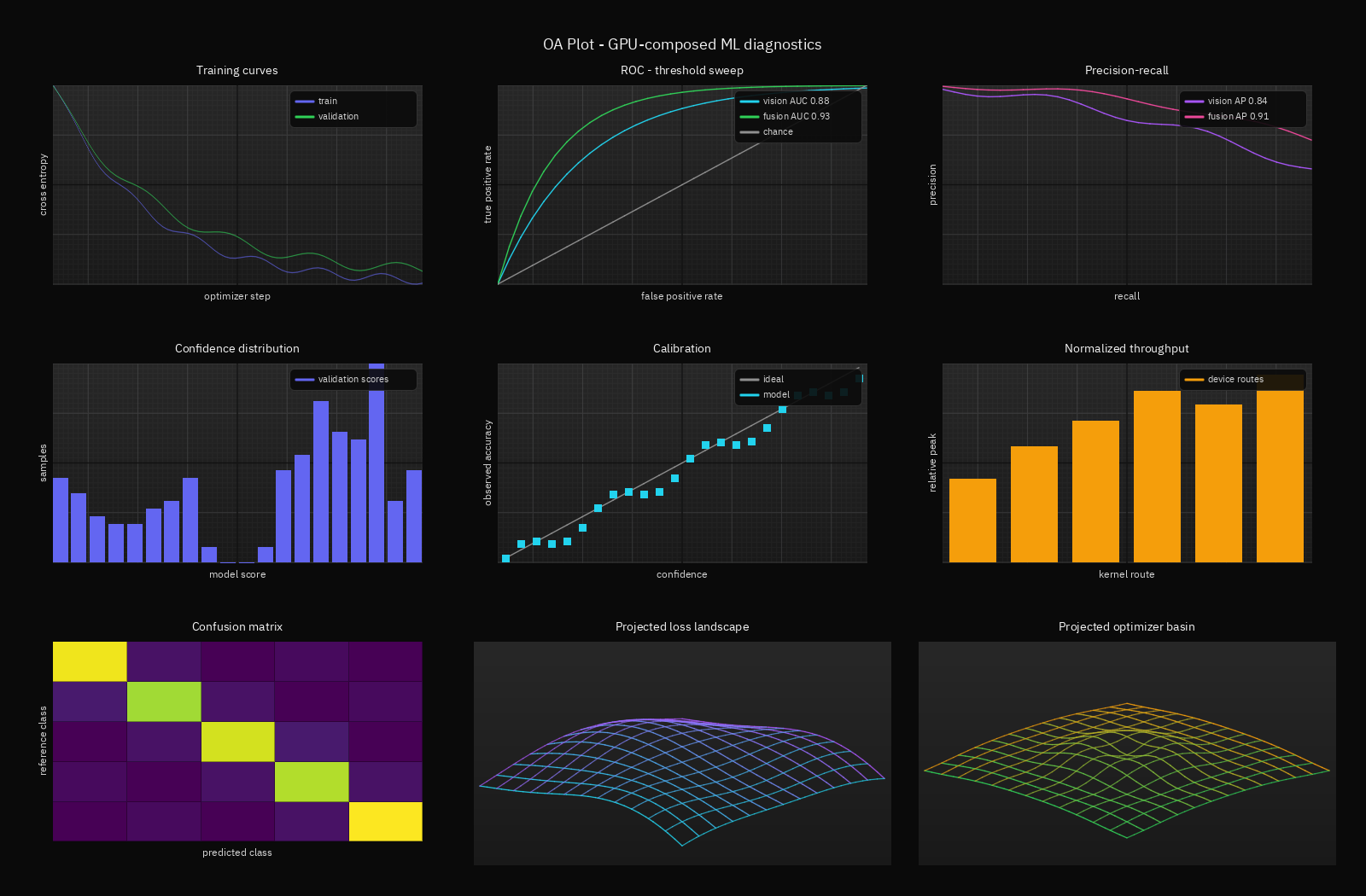
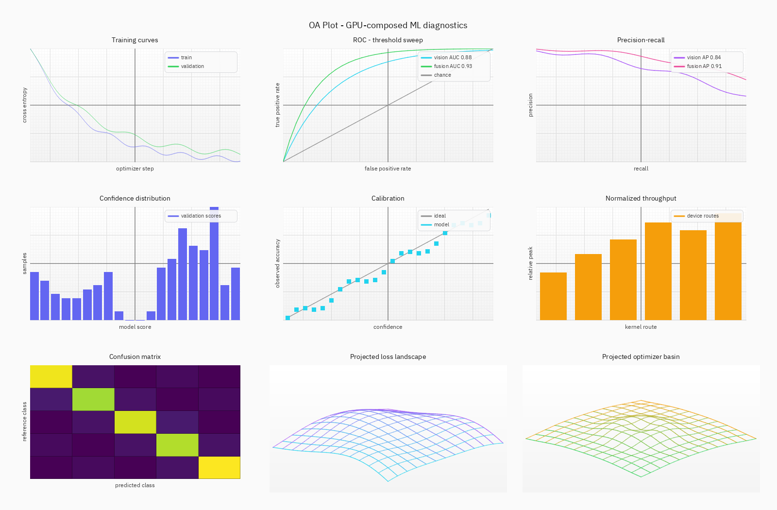
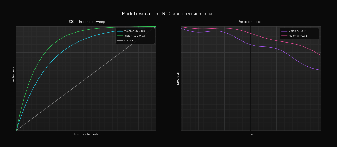
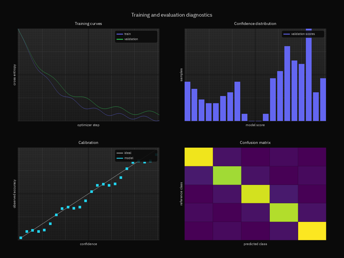
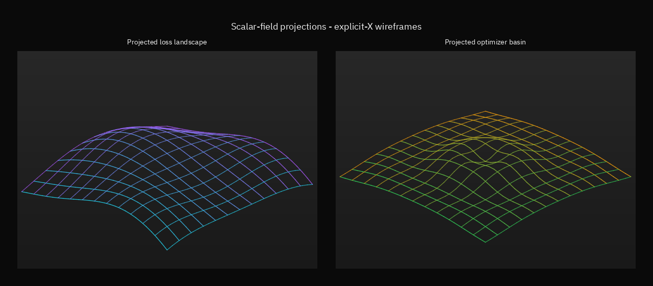
Six generated OA Plot examples